Least-Squares Method

Section 1A Bit of History

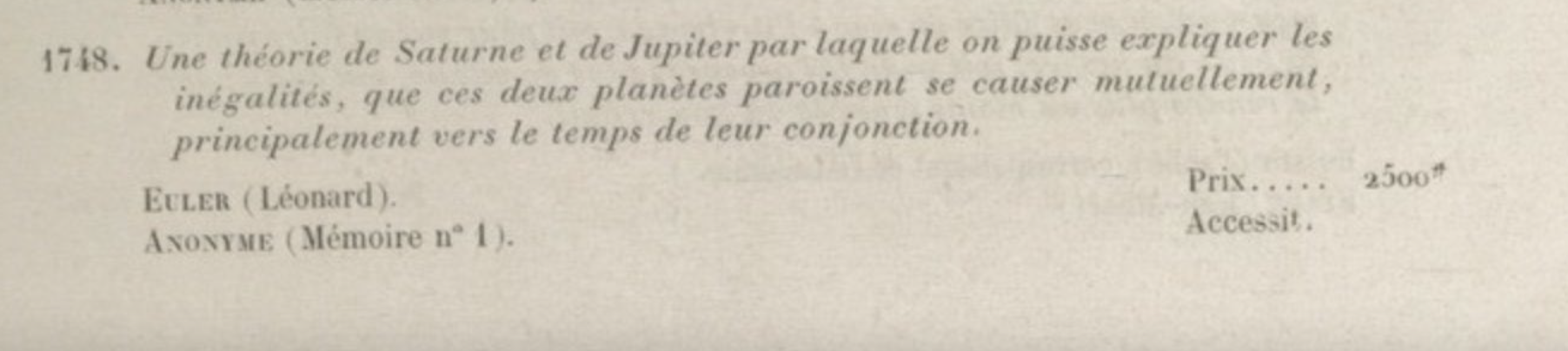
In 1748, the French Academy of Science posed the following challenge: use Newton's law of gravity to explain how Jupiter and Saturn cause each other to speed up or slow down. Euler came up with a response and won the prize. His response included an equation relating 8 orbital elements. To find the values of these 8 unknowns, he consulted the astronomical observation archive and found 75 observations — leading to the question:

How do you find 8 unknowns from 75 equations?

Figure 1. L. Euler was the winner of the 1748 French Academy of Science prize for explaining how Jupiter and Saturn cause each other to speed up or slow down.

Consider a simpler version of this problem, with two unknowns $X_1$ and $X_2$ and three equations:

Finding $X_1$ and $X_2$ is not straightforward. For example, the first two equations give $X_1 = 2$, $X_2 = 2$, but these values do not satisfy the third equation.

In 1805, the "mystery mathematician" (Legendre) came up with a systematic solution:

Find $X_1$ and $X_2$ that satisfy the equations with the least amount of error.

He defined the residual for each equation:

and aimed to minimize the sum of squared residuals:

This is the least-squares approach. Later, Gauss provided a probabilistic justification: the least-squares estimate gives the "most likely" values of $X_1$ and $X_2$ under a Gaussian assumption on the observation error — a justified assumption by the central limit theorem. The method is widely used because of its simplicity, flexibility, and because it only requires vector calculus and linear algebra.

Section 2Mathematical Formulation

Assume there are $n$ unknown variables $(X_1, \ldots, X_n)$ and $m$ observations $(Y_1, \ldots, Y_m)$ related by the linear model:

where $(W_1, \ldots, W_m)$ represent measurement noise. In compact matrix form:

For any estimate $\hat{X}$, define the residual $e = Y - H\hat{X}$. The least-squares estimate minimizes the squared norm of the residual:

We denote the objective function as:

Section 3Solution to the Least-Squares Problem

We use the first-order optimality condition to find candidate minimizers.

Applying the optimality condition $\nabla J(\hat{X}) = 0$ yields the normal equations:

When $H^\top H$ is invertible, the unique solution is:

3.1Uniqueness of the Solution

The matrix $H^\top H$ is invertible if and only if the null space of $H$ is empty, which requires all $n$ columns of $H$ to be linearly independent. Since $H$ is $m \times n$, this requires $m \geq n$ — at least as many measurements as unknowns.

Geometrically, each measurement is an inner product between a row $H_k$ of $H$ and the unknown $X$:

Invertibility requires measuring $X$ along at least $n$ linearly independent directions. When the null space of $H$ is empty, the minimizer is unique: if $\hat{X}$ and $X'$ are both minimizers, then $H\hat{X} = HX'$, and an empty null space forces $\hat{X} = X'$.

3.2Regularization Technique

When $H$ has a non-empty null space (too few independent measurements), there are infinitely many minimizers. We add a penalty on $\|\hat{X}\|$ and solve:

Section 4Application: Linear System Identification

Consider a discrete-time linear system:

where $z(t) \in \mathbb{R}^d$ is the state (e.g. deformation of an aircraft wing) and $A$ is unknown. We want to estimate $A$ from data $\{z(0), z(1), \ldots, z(t_f)\}$ by minimizing the one-step prediction error:

Setting $X = \text{vec}(A) \in \mathbb{R}^{d^2}$ (vectorize row by row), the dynamic update becomes $Y(t) = H(t)X + W(t)$ where $H(t)$ is a block-diagonal matrix built from $z(t)$. Stacking over all time steps gives $Y = HX + W$, and the least-squares solution applies directly.

The minimizer is unique when $H$ has $d^2$ linearly independent rows, which occurs when there are $d$ linearly independent state vectors in $\{z(0), \ldots, z(t_f - 1)\}$. This is the persistence of excitation condition — all modes of the system must be excited for successful identification.

Section 5Error Analysis

The estimation error from the least-squares algorithm depends directly on the minimum singular value of $H$. We first review the singular value decomposition.

5.1Mathematical Review: Singular Value Decomposition

For an $m \times n$ matrix $H$ with rank $r$, the SVD admits three equivalent representations:

1. Sum of rank-one matrices:

where $\sigma_i > 0$ are singular values, $u_i \in \mathbb{R}^m$ and $v_i \in \mathbb{R}^n$ are orthonormal vectors.

2. Compact matrix product:

where $U \in \mathbb{R}^{m \times r}$, $\Sigma \in \mathbb{R}^{r \times r}$ diagonal with positive entries, $V \in \mathbb{R}^{n \times r}$, and $U^\top U = V^\top V = I_{r \times r}$. Note $UU^\top$ projects onto the range of $H$, and $VV^\top$ projects onto the orthogonal complement of the null space of $H$.

3. Full matrix product: Extending $U$ and $V$ to square orthogonal matrices $\tilde{U}$ (m×m) and $\tilde{V}$ (n×n):

5.2Elementary Error Analysis

Working in the SVD basis (with $r = n$ for a unique minimizer), transform variables as:

In this basis, the observation model becomes $\beta_i = \sigma_i \alpha_i + \omega_i$ for $i = 1, \ldots, n$, and the minimizer takes the simple form $\hat{\alpha}_i = \beta_i / \sigma_i$. The estimation error then simplifies to:

Section 6Application: Auto-Regressive Models

Given time-series data $\{z(0), z(1), \ldots, z(t_f)\}$ (scalar), the linear auto-regressive model of order $n$ predicts future values from the last $n$ observations:

The unknown coefficients $a_1, \ldots, a_n$ can be estimated via least-squares once (6.1) is cast as $Y = HX + W$.

In practice, the model order is unknown. Statistical criteria such as the Akaike information criterion (AIC) provide principled ways to select the order that balances fit and overfitting. We do not cover these techniques in this course.

Section 7Application: Curve Fitting

Given time-series data $\{(t_k, Y_k)\}_{k=1}^m$, choose $n$ basis functions $\{\psi_1(t), \ldots, \psi_n(t)\}$ (e.g. polynomials, Fourier modes) and model each observation as:

Stacking gives $Y = HX + W$ where $H_{k,i} = \psi_i(t_k)$, and the unknowns $X = [X_1, \ldots, X_n]^\top$ are the expansion coefficients.

Section 8Programming Exercise

Track a target with constant but unknown acceleration. The position is $r(t) = [r_x(t), r_y(t)]$, and with constant acceleration:

The unknowns are $X = [a_x, b_x, c_x, a_y, b_y, c_y]^\top$ and the noisy observations are $Y_1(t) = r_x(t) + W_1(t)$, $Y_2(t) = r_y(t) + W_2(t)$.

Section 9Appendix: Mathematical Review on Gradients

We review two approaches to computing gradients of functions on vector spaces.

Gradient via partial derivatives. For $f: \mathbb{R}^n \to \mathbb{R}$, the gradient at $x$ is the $n$-vector of partial derivatives:

For example, $f(x) = x_1^2 + \cdots + x_n^2$ gives $\nabla f(x) = x$.

Geometric (coordinate-free) approach. This method works on any vector space $V$ with inner product $\langle \cdot, \cdot \rangle$. Define the directional derivative of $f: V \to \mathbb{R}$ at $x$ along direction $u$ as:

The gradient $\nabla f(x) \in V$ is the unique vector satisfying:

The gradient points in the direction of steepest ascent.