Week 4 — Minimum MSE Estimation

Section 1Introduction to MSE Estimation

Consider the following estimation setup: a hidden random variable $X \in \mathbb{R}^n$, an observation $Y \in \mathbb{R}^m$, and an estimator $\hat{X} \in \mathbb{R}^n$ which is a function of $Y$ designed to approximate $X$. In the MSE estimation framework, the estimator is obtained by minimizing:

$$\min_{\hat{X} \in \mathcal{V}_Y} E\bigl[\|X - \hat{X}\|^2\bigr]$$

where $\mathcal{V}_Y$ is the space of estimators we search over. In this lecture we consider two choices:

Linear estimators: $\mathcal{V}_Y = \{KY + b \;;\; K \in \mathbb{R}^{n \times m},\; b \in \mathbb{R}^n\}$
All estimators: $\mathcal{V}_Y = \{f(Y) \;;\; f : \mathbb{R}^m \to \mathbb{R}^n\}$

We also identify the setting where the linear estimator is optimal among all estimators.

Section 2Minimum Linear MSE Estimation

2.1Scalar Case

Assume both $X$ and $Y$ are scalar. The MSE minimization over $k, b \in \mathbb{R}$ is:

$$\min_{k,b} \; E\bigl[(X - kY - b)^2\bigr]$$

Expanding and completing the square using the rules of covariance and expectation:

$$E[(X - kY - b)^2] = \text{var}(X) - \frac{\text{cov}(X,Y)^2}{\text{var}(Y)} + \left(k - \frac{\text{cov}(X,Y)}{\text{var}(Y)}\right)^2 \text{var}(Y) + (E[X] - kE[Y] - b)^2$$

This is minimized by:

$$k^* = \frac{\text{cov}(X,Y)}{\text{var}(Y)}, \qquad b^* = E[X] - k^* E[Y]$$

Minimum Linear MSE Estimate (Scalar)

$$\hat{X}^* = E[X] + \frac{\text{cov}(X,Y)}{\text{var}(Y)}\bigl(Y - E[Y]\bigr)$$

The minimum MSE achieved is:

$$E[e^2] = \text{var}(X) - \frac{\text{cov}(X,Y)^2}{\text{var}(Y)}$$

where $e = X - \hat{X}^*$.

1.

The formula depends only on the first and second moments of $X$ and $Y$, and their covariance — not on the full joint distribution. It is the optimal linear estimate even when $X$ and $Y$ do not have a linear relationship.

2.

The estimate has a feedback-error correction form: the prior guess $E[X]$ is corrected by gain $k^*$ times the innovation $Y - E[Y]$.

3.

The minimum MSE $E[e^2]$ equals the prior uncertainty $\text{var}(X)$ reduced by a term proportional to the correlation between $X$ and $Y$.

4.

When $\text{cov}(X,Y) = 0$, we have $\hat{X}^* = E[X]$ — the observation provides no information.

Example 2.1 · Gaussian with Additive Noise

Let $X \sim \mathcal{N}(\mu, \sigma^2)$ and $Y = X + W$ with $W \sim \mathcal{N}(0, r^2)$ independent of $X$. Then:

$$k^* = \frac{\sigma^2}{\sigma^2 + r^2}, \qquad \hat{X} = \frac{\sigma^2}{\sigma^2 + r^2} Y + \frac{r^2}{\sigma^2 + r^2}\mu$$

This is a convex combination of the observation $Y$ and the prior mean $\mu$. When $r/\sigma \ll 1$ (low noise), $\hat{X} \approx Y$. When $r/\sigma \gg 1$ (high noise), $\hat{X} \approx \mu$. The minimum MSE is:

$$E[(X - \hat{X})^2] = \frac{\sigma^2 r^2}{\sigma^2 + r^2}$$

2.2Vector Case

For $X \in \mathbb{R}^n$ and $Y \in \mathbb{R}^m$, we minimize over $K \in \mathbb{R}^{n \times m}$ and $b \in \mathbb{R}^n$. Writing the error $e := X - KY - b$ and the MSE as:

$$E\bigl[\|e\|^2\bigr] = \text{Tr}(\text{Cov}(e)) + \|E[e]\|^2$$

Expanding the error covariance and completing the square in $K$:

$$\text{Cov}(e) = \text{Cov}(X) - \text{Cov}(X,Y)\text{Cov}(Y)^{-1}\text{Cov}(Y,X) + (K - K^*)^\top \text{Cov}(Y)(K - K^*)$$

where $K^* = \text{Cov}(X,Y)\text{Cov}(Y)^{-1}$. The square-norm of the expectation of the error is simplified as

$$\|E[e]\|^2 = \|E[X]-KE[Y] - b\|^2$$

concluding the following simplified expression for the MSE

$$E\bigl[\|e\|^2\bigr] = \text{const.} + \text{Tr}((K - K^*)^\top \text{Cov}(Y)(K - K^*)) + \|E[X]-KE[Y] - b\|^2$$

The optimal gain and bias are:

Minimum Linear MSE Estimate (Vector)

$$K^* = \text{Cov}(X,Y)\,\text{Cov}(Y)^{-1}, \qquad b^* = E[X] - K^* E[Y]$$ $$\hat{X}^* = E[X] + K^*\bigl(Y - E[Y]\bigr)$$

The optimal error $e^* = X - \hat{X}^*$ satisfies $E[e^*] = 0$ and:

$$\text{Cov}(e^*) = \text{Cov}(X) - \text{Cov}(X,Y)\,\text{Cov}(Y)^{-1}\,\text{Cov}(Y,X)$$

Example 2.2 · Kalman Gain

Let $X \sim \mathcal{N}(\mu, \Sigma)$ and $Y = HX + W$ with $W \sim \mathcal{N}(0, R)$ independent of $X$. Using $\text{Cov}(X,Y) = \Sigma H^\top$ and $\text{Cov}(Y) = H\Sigma H^\top + R$:

$$K^* = \Sigma H^\top(H\Sigma H^\top + R)^{-1}$$

$$\hat{X} = \mu + K^*(Y - H\mu)$$

The matrix $K^*$ is the Kalman gain — this formula appears directly in the Kalman filter update equations. The error covariance is:

$$\text{Cov}(e) = \Sigma - \Sigma H^\top(H\Sigma H^\top + R)^{-1}H\Sigma$$

The MSE of the optimal estimate is $E[\|e\|^2] = \text{Tr}(\text{Cov}(e))$.

Example 2.3 · Error Covariance Ellipse

Let $X = [X_1, X_2]^\top \sim \mathcal{N}(0, I)$ and $Y = h_1 X_1 + h_2 X_2 + W$ with $W \sim \mathcal{N}(0, r^2)$. Then:

$$\begin{bmatrix}\hat{X}_1 \\ \hat{X}_2\end{bmatrix} = \frac{1}{h_1^2 + h_2^2 + r^2}\begin{bmatrix}h_1 Y \\ h_2 Y\end{bmatrix}$$

$$\text{Cov}(X - \hat{X}) = I - \frac{1}{h_1^2 + h_2^2 + r^2}\begin{bmatrix}h_1^2 & h_1 h_2 \\ h_1 h_2 & h_2^2\end{bmatrix}$$

The uncertainty ellipse $\{x : x^\top \text{Cov}(X-\hat{X})^{-1} x = 1\}$ grows in directions where the error covariance is large. Study the effect of $[h_1, h_2]$ on the ellipse in the code demonstration.

Exercise 1

Relate the optimal linear MSE estimate to the regularized least-squares problem.

(a) Show that the solution to $\min_{\hat{X}} \|Y - H\hat{X}\|^2 + \lambda\|\hat{X}\|^2$ equals the optimal linear MSE estimate when $X \sim \mathcal{N}(0, \frac{1}{\lambda}I)$ and $W \sim \mathcal{N}(0,I)$. Use the identity $(I + UV)^{-1}U = U(I + VU)^{-1}$.
(b) Show that the solution to $\min_{\hat{X}} (Y - H\hat{X})^\top R^{-1}(Y - H\hat{X}) + (\hat{X} - \mu)^\top \Sigma^{-1}(\hat{X} - \mu)$ equals the optimal linear MSE estimate when $X \sim \mathcal{N}(\mu, \Sigma)$ and $W \sim \mathcal{N}(0, R)$.

Section 3Minimum MSE Estimation

Can we achieve a lower MSE with a nonlinear estimator $\hat{X} = f(Y)$? To answer this, we first need conditional probabilities and conditional expectations.

3.1Conditional Probability

The conditional probability of event $A$ given event $B$ is denoted $P(A|B)$. Using the identity $P(A \text{ and } B) = P(B)P(A|B) = P(A)P(B|A)$, we obtain Bayes' law:

$$P(A|B) = \frac{P(A)\,P(B|A)}{P(B)}$$

Example 3.1 · Smoking and Cancer

Let $A$ = patient has lung cancer, $B$ = patient smokes. Suppose $P(B|A) = 0.8$, $P(A) = 0.05$, $P(B) = 0.2$. Then:

$$P(A|B) = \frac{0.05 \times 0.8}{0.2} = 0.2$$

The probability of lung cancer given smoking is 20%. (Numbers are illustrative.)

Exercise 2

A family has two children. Each child is equally likely to be a girl or boy. You observe that one child is a girl. What is the probability that the other child is also a girl?

3.2Conditional Probability Density Functions

For random variables $X$ and $Y$ with joint density $p_{X,Y}(x,y)$, the conditional density of $X$ given $Y$ satisfies:

(3.1)$$p_{X,Y}(x,y) = p_Y(y)\, p_{X|Y}(x|y)$$

Interchanging $X$ and $Y$ and applying Bayes' law for densities:

$$p_{X|Y}(x|y) = \frac{p_X(x)\, p_{Y|X}(y|x)}{p_Y(y)}$$

Example 3.2

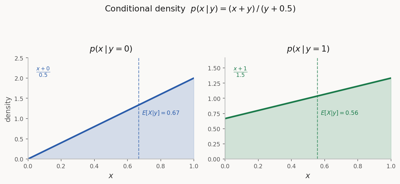
For $p(x,y) = x + y$ on $[0,1]^2$ with marginal $p_Y(y) = y + \frac{1}{2}$:

$$p_{X|Y}(x|y) = \frac{x + y}{y + \frac{1}{2}}$$

The figure below shows this conditional density for four values of $y$. As $y$ increases, the distribution shifts toward larger $x$ values and becomes more uniform.

Figure 1. The conditional density $p_{X|Y}(x|y)$ for $y = 0, 0.25, 0.5, 1$.

Exercise 3

Show that if $X$ and $Y$ are independent, then $p_{X|Y}(x|y) = p_X(x)$ and $p_{Y|X}(y|x) = p_Y(y)$.

3.3Conditional Expectation

The conditional expectation of $X$ given $Y = y$ is:

$$E[X|Y=y] = \int_{-\infty}^\infty x\, p_{X|Y}(x|y)\,dx$$

More generally, $E[f(X)|Y=y] = \int f(x)\, p_{X|Y}(x|y)\,dx$. Dropping $=y$, the conditional expectation $E[X|Y]$ is a random variable — a function of $Y$.

Example 3.3

For $p(x,y) = x+y$ on $[0,1]^2$:

$$E[X|Y] = \int_0^1 x \cdot \frac{x+Y}{Y+\frac{1}{2}}\,dx = \frac{\frac{Y}{2} + \frac{1}{3}}{Y + \frac{1}{2}}$$

$$E[X^2|Y] = \int_0^1 x^2 \cdot \frac{x+Y}{Y+\frac{1}{2}}\,dx = \frac{\frac{Y}{3} + \frac{1}{4}}{Y + \frac{1}{2}}$$

Rules for Conditional Expectation

$E[X|Y]$ is a function of $Y$: there exists $\hat{f}$ such that $E[X|Y] = \hat{f}(Y)$.
Linearity: $E[\alpha X + \beta Z|Y] = \alpha E[X|Y] + \beta E[Z|Y]$.
$E[Xf(Y)|Y] = f(Y)E[X|Y]$ — any function of $Y$ is treated as a constant.
$E[X|Y] = E[X]$ when $X$ and $Y$ are independent.
Tower property: $E[E[X|Y]] = E[X]$.
$E[E[X|Y,Z]|Y] = E[X|Y]$.

Exercise 4

Use the definition of conditional expectation to prove rule (5): $E[E[X|Y]] = E[X]$.

Exercise 5

Let $X \sim \mathcal{N}(0,1)$ and $Y = X + W$ with $W \sim \mathcal{N}(0,r^2)$ independent of $X$, so $p_{Y|X}(y|x) = \frac{1}{\sqrt{2\pi r^2}}e^{-(y-x)^2/(2r^2)}$.

(a) Show that $p_{X|Y}(x|y) = \frac{1}{\sqrt{2\pi\sigma^2}}e^{-(x - \frac{y}{1+r^2})^2/(2\sigma^2)}$ where $\sigma^2 = \frac{r^2}{1+r^2}$.
(b) Use part (a) to find $E[X|Y]$.
(c) Compare with the optimal linear MSE estimate.

3.4Conditional Expectation as Minimum MSE Estimate

We now solve $\min_f E[(X - f(Y))^2]$ over all functions $f$. Conditioning on $Y$:

$$E[(X - f(Y))^2|Y] = E[X^2|Y] - E[X|Y]^2 + (f(Y) - E[X|Y])^2$$

Taking expectations of both sides:

$$E[(X - f(Y))^2] = \underbrace{E\bigl[E[X^2|Y] - E[X|Y]^2\bigr]}_{\text{independent of }f} + \underbrace{E\bigl[(f(Y) - E[X|Y])^2\bigr]}_{\geq\, 0,\;\text{minimized when }f(Y) = E[X|Y]}$$

Summary · MSE Estimation

Optimal nonlinear estimate (over all functions $f$):

$$\hat{X} = E[X|Y] = \int x\, p_{X|Y}(x|Y)\,dx$$

Optimal linear estimate (over $\hat{X} = KY + b$):

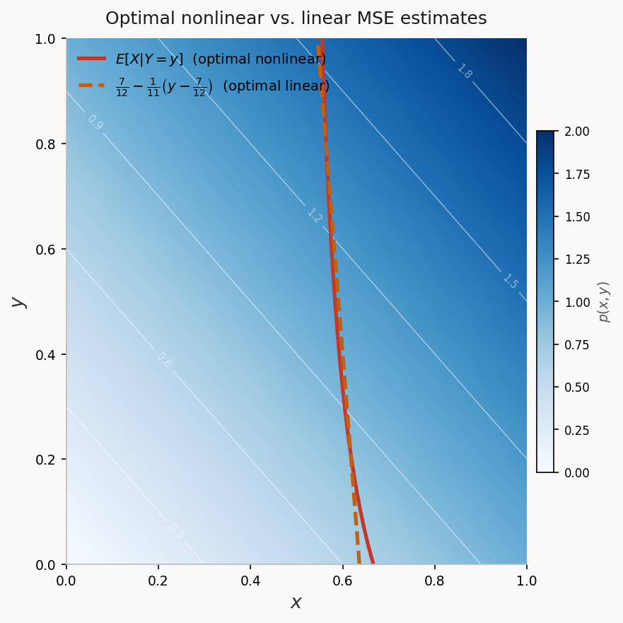
$$\hat{X} = E[X] + K^*(Y - E[Y]), \qquad K^* = \text{Cov}(X,Y)\,\text{Cov}(Y)^{-1}$$

Example 3.4 · Comparison of Estimators

For $p(x,y) = x+y$ on $[0,1]^2$, the optimal (nonlinear) estimate is:

$$E[X|Y] = \frac{\frac{Y}{2} + \frac{1}{3}}{Y + \frac{1}{2}}, \qquad \text{MSE} = \frac{1}{12} - \frac{1}{144}\log(3) \approx 0.07570$$

The optimal linear estimate is:

$$\hat{X} = \frac{7}{12} - \frac{1}{11}\left(Y - \frac{7}{12}\right), \qquad \text{MSE} = \frac{5}{66} \approx 0.07576$$

The two MSE values are remarkably close, with the nonlinear estimator offering only a marginal improvement — consistent with the small negative correlation between $X$ and $Y$.

Comparison of conditional expectation and optimal linear estimate

Figure 2. The conditional expectation $E[X|Y]$ (solid red) vs. the optimal linear MSE estimate (dashed orange), overlaid on the joint density $p(x,y) = x+y$.

Section 4Jointly Gaussian Setting

Computing the conditional expectation is generally hard. An important tractable case is when $X$ and $Y$ are jointly Gaussian, i.e., $Z = [X, Y]^\top$ has a Gaussian density. In this case, the conditional expectation is linear and coincides with the optimal linear MSE estimate.

Key Result · Jointly Gaussian

If $X$ and $Y$ are jointly Gaussian, then:

$$E[X|Y] = KY + b, \qquad K = \text{Cov}(X,Y)\,\text{Cov}(Y)^{-1}, \quad b = E[X] - KE[Y]$$

Moreover, the conditional density $p_{X|Y}(x|y)$ is Gaussian $\mathcal{N}(KY+b,\, P)$ where:

$$P = \text{Cov}(X) - \text{Cov}(X,Y)\,\text{Cov}(Y)^{-1}\,\text{Cov}(Y,X)$$

Proof Sketch

Define $\hat{X} = KY + b$ and error $e = X - \hat{X}$. Both are Gaussian. The estimate formula implies $\text{Cov}(e, Y) = 0$, and since $e$ and $Y$ are Gaussian, they are independent. Therefore $e$ and $\hat{X}$ are independent. Since $X = \hat{X} + e$ with $e$ independent of $\hat{X}$ and $e \sim \mathcal{N}(0, P)$, conditioning on $Y$ gives $X|Y \sim \mathcal{N}(\hat{X}, P)$. $\square$

This result is fundamental: in the Gaussian setting, the linear estimator is globally optimal, and we never need to search for nonlinear improvements.

Section 5Programming Exercise: Nonlinear Estimation

Let $X(0) \sim \mathcal{N}(0, P)$ and $X(1) = X(0) + U$ where $U = \pm 1$ with equal probability, independent of $X(0)$. The observation is $Y = X(1) + W$ with $W \sim \mathcal{N}(0, R)$ independent of everything else.

Deliverables

(a) Write code generating $N$ i.i.d. samples $\{(X(1)_i, Y_i)\}_{i=1}^N$. Plot a scatter plot with $P = 0.1$, $R = 0.4$.
(b) Derive the best linear MSE estimator $\hat{f}_{\text{lin}}(Y)$ as a formula in $P$ and $R$. Overlay the estimator on the scatter plot.
(c) Extend the search to $\mathcal{V} = \{c_0 + c_1\psi_1(Y) + \cdots + c_m\psi_m(Y)\}$. Use the optimality conditions to show the best estimator in $\mathcal{V}$ is:
$$E[X(1)] + \text{Cov}(X, \psi(Y))\,\text{Cov}(\psi(Y))^{-1}\bigl(\psi(Y) - E[\psi(Y)]\bigr)$$
(d) With $\psi(Y) = [Y, Y^3]^\top$, approximate the estimator numerically using sample means and covariances. Call it $\hat{f}_{\text{cubic}}(Y)$ and add to the scatter plot.
(e) Repeat with $\psi(Y) = [Y, \text{sgn}(Y)]^\top$ where $\text{sgn}(Y) = \mathbf{1}_{Y > 0}$. Call it $\hat{f}_{\text{sgn}}(Y)$ and add to the scatter plot.
(f) Numerically compare the MSE for all three estimators. Which performs best?